Multi-Star Autofocus for High Resolution Telescope Imaging
Frank Freestar8n July, 2019
Introduction
Everyone knows that good focus is important for high
quality astro-imaging – but sometimes there is a disconnect
between how focus is measured and the actual quality of the image. In
addition, there may be concerns for drift in focus without a good
understanding of how a given drift impacts image quality. This write
up intends to address these issues by describing a form of autofocus
based on the measurement of star quality as you go through focus –
along with a statistical analysis of the errors involved and how they
translate to uncertainties in the focus performance. This is
important because any measurement lacks value if you have no idea of
its inherent uncertainty – particularly if you are trying to
assess the significance of small changes in such a measurement.
Focus is easy to understand in simple geometric optics,
but when you are dealing with a realistic astro-imaging situation
with seeing, aberrations and guiding errors – even the
definition of 'in focus' becomes elusive. Some people rely on
indirect methods to determine focus, such as a Bhatinov mask, but
such methods aren't directdly relatable to the quality of the image.
Instead it assumes that when some separate optical properties are met
– the actual image will be optimal. But not only does this end
up decoupled from the actual quality of the image – it gives no
indication of how sensitive the final focus is relative to the
optimum.
This write up describes a form of through-focus,
multi-star autofocus based on the changing size of stars in the
actual image as you go through focus – and it details how to
apply the measured uncertainties in star size to a corresponding
uncertainty in focus. This satisfies the desire to have a sense of
possible error in focus associated with each focus measurement –
and allows an assessment of when a given focus change is significant
or not. And the shape of the through-focus curve tells you how much a
given amount of focus error actually impacts the quality of the image
at the time of each focus measurement, with a corresponding
assessment of seeing quality at focus.
Overview of existing autofocus methods
One of the first autofocus systems for amateur astro
imaging was FocusMax in around 2001 (https://www.focusmax.org/
), which used a single bright star and a pre-characterized model of
how star size changed with focus for a given imaging system. The goal
was to be fast and accurate – but required moving away from the
imaging target to a nearby bright star for focus. It is in the class
of focusing methods that assumes a model for how focus behaves –
and based on that model makes measurements of a star near focus and
deduces the true focus without actually going through focus.
Recently more sensitive cameras have allowed focusing
based on multiple stars in view of the actual imaging target –
so there is no slew required to a bright star. Sequence Generator
Pro, or SGP (http://mainsequencesoftware.com/Products/SGPro
) is a popular example that measures the size of multiple field stars
as the system moves through focus – and uses geometric
heuristics on the resulting plots to estimate optimal focus.
With both FocusMax and SGP the star size is based on a
half-flux diameter or radius estimate – and like any star size
heuristic it may be challenged when the star is far enough out of
focus that it becomes 'donut' shaped due to the secondary
obstruction, or when aberrations cause it to be distorted or vary in
size and shape across the field.
My approach: Multi-Star autofocus with error
estimates and a weighted parabolic fit
Half-flux diameter is often regarded as a robust measure of star
size – but it has the disadvantage that it can be very
sensitive to the assumed background level around the star if the star
has a lot of energy spread out into the 'wings.' This can lead to
uncertainty as you go through focus – and a large variation in
star size with star intensity. An ideal star size measurement should
be independent of star intensity and the resulting through-focus
curve of star size should be well shaped and have a clear minimum.
I use a Moffat fit to each star that allows for ellipticity and
arbitrary orientation. From the resulting Moffat fit I can calculate
the fwhm directly from the model parameters. I find this to behave
very well for SCT autofocus – and it generates nice parabolic
curves of star size through focus.
My main imaging work is with EdgeHD11 at f/7 or f/10 – and I
focus using a stepper motor on the primary mirror focusing knob. This
requires about ½ turn of the knob for backlash compensation –
but is extremely simple and quite repeatable – as you can tell
directly from a series of autofocus runs.
I typically capture focus images binned x2 to about 0.8” per
binned pixel - and two-second exposures – with 7 steps through
focus generating a curve that goes from about 2” min fwhm to 6”
or so – and a nice parabolic bowl shape close to focus and far
from where any donut stars would appear.
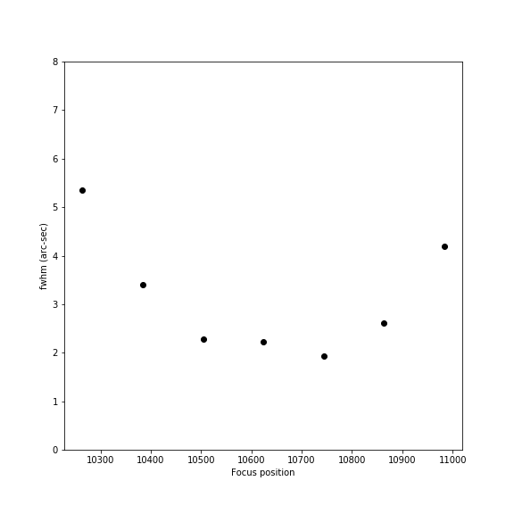
Here is a raw view of the points in such an autofocus run:

The
overall shape of the curve is clear – but the slight jump in
the central point makes it hard to know the exact location of best
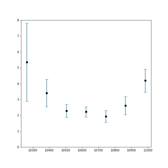
focus. But each fwhm measurement is based on many stars in the image
– and the standard deviation of fwhm at each point can be
plotted as error bars on those points:

This
gives a much better idea of the weight that should be assigned to
each point – and you can see that the central point, which
looks a bit 'wrong', is not particularly far off the parabola given
the uncertainty of it and its adjacent points. The uncertainty of
the point on the far left is very high – perhaps due to slight
motion of the mount, or wind, during the exposure. The goal here is
to take a quick sweep through focus and take as little time as
possible – and allow anomalous measurements to happen with the
understanding they will have correspondingly less weight to the final
measurement due to their larger error bars.
It is standard statistical practice to do a model fit that is
weighted by the uncertainty at each point so that the most likely
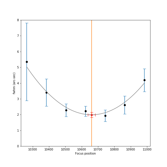
parabola fitting the data can be calculated:

Here the gray curve is the best fitting parabola to the
data, the orange vertical line is the location of best focus, and the
red error bars indicate the resulting errors both in the focus
position and the minimum fwhm for the focus curve. You can see that –
based on the data and measured uncertainties – the resulting
error in focus position is very small and in the flat part of the
focus curve. You can also see that the point on the left with a large
error bar contributes correspondingly less weight to the curve –
allowing the points near focus with less error to play a stronger
role.
Ideally the errorbars would represent the true,
inherent uncertainties in each well-defined measurement of star size.
In that case, the error bars should be much smaller since they
represent the standard error of the mean, rather than the standard
deviation. But I find that if I use the standard error of the mean,
and divide the standard deviation by sqrt(NStars) – the
resulting error bars are too small and don't faithfully represent the
uncertainty of each focus measurement. So – the use of
standard deviation here isn't perfect – and likely
overestimates the error – but it doesn't affect the overall fit
very much. But whatever method is used to measure the image quality
– it's important to have some idea of the uncertainty in each
measurement so a weighted fit can be performed that yields
corresponding uncertainties in the fit model parameters.
I do autofocus runs approximately every 40 minutes –
and since each run tells you both the current focus and the shape of
the curve – you can tell how much focus is drifting and how
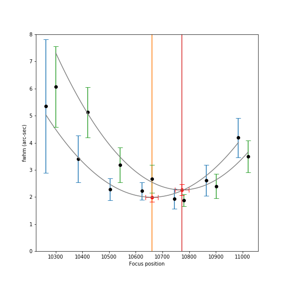
much impact it has on bloating of the fwhm. Here is an overlapping
view of two focus curves 40 minutes apart:

Here you can see several things all at once. First, the
focus has changed from about 10660 to 10770 – or a drift of 110
steps. At the same time, the min fwhm has increased a bit –
indicating that seeing has gotten worse – though the change in
fwhm is not very large compared to the estimated error in fwhm shown
by the red error bars. But you can only tell this change in seeing if
you go through focus and measure the parabola. Simply measuring a
change in fwhm over time could be due to pure focus drift or pure
seeing – or a mixture of both. Comparing the two separate
through-focus curves lets you know exactly what is happening.
You can also estimate how significant the focus drift
of 110 steps is – by viewing it in the context of the gray
parabolic fit. This graph shows a coincidental increase of fwhm due
to seeing that causes the second red dot of perfect focus to land
directly on the previous focus curve – but if there had been no
change in seeing the second gray curve would be purely translated to
the right from the original curve. Based on the gray curve itself,
the change in fwhm due to focus drift would be about 2.0 to 2.2”.
This is a bit high – but keep in mind that if the drift is
steady then most of the images captured in the time between focus
measurements will be in the flat part of the parabolic curve –
hence the stacked images will only be slightly bloated by the few
later exposures that are higher on the parabolic curve.
Math behind the fit and error analysis
The mathematics behind the uncertainty analysis and model fit is
fairly straightforward and can be found in books on statistical data
analysis.
The fwhm near focus is assumed to follow a simple parabolic model:

where w is the mean star width, p is the focus step position, p0
is the optimal focus position, and w0 is
the star width at optimal focus.
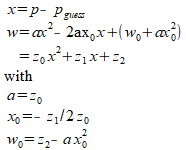
This equation can be rewritten as a simple polynomial
that can be solved for its coefficients:

At this point p is the raw focuser step position, which
could be a very large number in the thousands – but the
numerics of the solution are more robust if everything is centered
close to focus so that the x-axis values near the parabola are near
zero. So we provide an initial guess of the focus and shift the
parabola based on that offset as follows:

The above shows how the original model is represented by a pure
polynomial – and how to convert the best fit polynomial
coefficients to the desired model parameters (focus position,
curvature and minimum fwhm). If the image at each step through focus
is analyzed and fwhm is measured for many stars, then the error bars
result from the mean fwhm and associated standard deviation about
that mean. Thus for each step along the focus curve you have fwhm[i]
and sigma[i] – and all values are empirical, based on direct
measurements of stars in the image – instead of a model.
There are numerous statistical packages for performing a fit such
as this, and I use Python and Numpy. The process is as follows:
Do a polynomial fit of order 2, weighted by 1/variance, and
generate the covariance matrix. The diagonal elements of the
covariance matrix are the variances of the corresponding coefficients
in the polynomial fit. But you need to handle the actual covariance
of terms properly since the uncertainties in the polynomial terms are
correlated. Once you have the polynomial coefficients and the
covariance matrix you can determine the best focus position and min
fwhm – along with their uncertainties.
Here is the corresponding Python/Numpy code. Note one subtlety
that the polyfit routine wants the weights specified as 1/sigma
rather than 1/variance – even though under the covers the
weighting will happen using variance.
z,
cov = np.polyfit(x2,
y, 2, w=1/sigma, cov=True)
#
z has the fit terms as z[0]x^2 + z[1]x + z[2]
covab
= cov[0][1] # covariance of z[0] with z[1] for use later
cov2
= np.sqrt(np.diag(cov))
# standard deviation of the z[i] coefficients
BestFocus
= -0.5*z[1]/z[0] # note this is still relative to p_guess
#
Once you know the x value of best focus, you can find the minfwhm
there:
minfwhm
= z[0]*BestFocus**2 + z[1]*BestFocus + z[2]
But calcuating the estimated error
in focus requires including the covariance terms since the z[1]
and z[0] terms are being divided. If the uncertainties of those two
fit parameters are correlated – and in general they will be –
then the net uncertainty won't simply add in quadrature and you need
to include a correction for the covariance.
Error in bestfocus = error in
-0.5*z[1]/z[0]. First find the fractional error in focus as the
fractional change in the z[1]/z[0] ratio. Then multiply by the
BestFocus value to get the true error in focus.
The full expression for the sigma fwhm
is more complicated with the covariance terms – but I assume
they are relatively small and I ignore them – and just use the
standard deviation of the z[2] coefficient itself.
focerrfrac
= sqrt((cov2[0]/z[0])**2 + (cov2[1]/z[1])**2 - 2*covab/(z[0]*z[1]))
focerr
= abs(BestFocus*focerrfrac)
fwhmsig
= cov2[2]
Overall I think this is a good and fast
way to find focus – and it allows you to see the final estimate
in the context of the actual shape of the focus curve – along
with an estimate of the error in the estimate. This give much more
insight into how sensitive your system is to focus drift – and
how often you need to re-focus. A key point is that you don't need
to take many measurements through focus – and you don't need to
measure far from focus where the star spots become fainter and take
on problematic shapes.
There is no need to be concerned about
re-focusing based on some estimate of the “central focus zone”
or CFZ of your system – because the parabolic shape tells you
everything you need to know in terms of how much the star bloats as a
result of focus error. Expressions for CFZ are usually based on
diffraction limited imaging – whereas deep sky imaging tends to
be far from diffraction limited and is more tolerant of focus drift.
In addition, if you know the rate of
drift and you know the shape of the parabola, most of images over
time will be in the flat part of the parabola with little impact on
fwhm. Only the later images will drift up the curve and bloat much.
And when you stack a series of such images, the contribution of bloat
to the final stack is much less then people tend to think.
I provide a tool for estimating the
impact of such drift here:
https://freestar8n.shinyapps.io/FranksFocusDrift/
and I describe it in more detail here:
https://www.cloudynights.com/topic/623265-focus-drift-analysis-in-stacked-exposures/
